Linear, Radial & Conic Gradients in Python from Scratch
An RGB value can be thought of as a point in 3D space. Given two RGB values, we can "move" from one to the next—that is, we can stretch a line between the two colors and place evenly spaced points. Each of these points can be interpreted as an RGB value which we can plot. If we plot all of these points in a line we get a smooth gradient of color. This process is called linear interpolation, commonly abbreviated as "lerping."
import numpy as np
from PIL import Image

def gradient(c1, c2, t):
    assert 0 <= t <= 1
    return tuple(np.clip(c1 + (c2-c1)*t, 0, 255).astype(int))

img = Image.new('RGB', (256, 256))
img.putdata([gradient(
    np.array([255,   0,   0]),
    np.array([  0,   0, 255]), x/256
) for x in range(256)]*256)
img.save('out.png')
The above Python code should yield the image out.png featured below (but with a different proportion and resolution) which shows a smooth transition (AKA a gradient) from the color red to blue. When given two colors the gradient function selects a point on the line stretched from c1 to c2 depending on the timestep t, a number from 0 to 1. It does this by calculating the distance from c1 to c2 and multiplying it by the t—note that c1 + (c2-c1)*0 == c1 and c1 + (c2-c1)*1 == c2. It ensures that the RGB components are clamped/clipped between 0 and 255 and that we return integers and not floats. The timestep we pass it is the X position of the pixel we're calculating the gradient for, scaled to be between 0 and 1.

We can have gradients with arbitrary "stops" where each stop indicates a position and color. We find the stop with the greatest position smaller than t, such that t lies between this stop and the next. We then lerp these two colors but with a timestep that is scaled to be between the two stops.
import numpy as np
from PIL import Image

def lerp(c1, c2, t):
    assert 0 <= t <= 1
    return np.clip(c1 + (c2-c1)*t, 0, 255).astype(int)

def gradient(stops, t):
    assert 0 <= t <= 1
    assert len(stops) >= 2
    for loc, _ in stops:
        assert 0 <= loc <= 1
    assert stops[0][0] == 0
    assert stops[-1][0] == 1
    for i in range(len(stops)-1):
        assert stops[i][0] <= stops[i+1][0]

    i = 0
    while stops[i+1][0] < t:
        i += 1
    loc1, c1 = stops[i]
    loc2, c2 = stops[i+1]

    return tuple(lerp(c1, c2, (t-loc1) / (loc2-loc1)))

img = Image.new('RGB', (256, 256))
img.putdata([gradient([
    ( 0, np.array([255,   0,   0])),
    (.5, np.array([255, 255, 255])),
    (.7, np.array([255, 255, 255])),
    ( 1, np.array([  0,   0, 255])),
], x/256) for x in range(256)]*256)
img.save('out.png')
The majority of the gradient() function is taken up by assertions to ensure data validity. It takes a list of tuples where the first element represents the position from 0 to 1 and the second is the associated color. Note how the technique of putting two stops of identical color directly adjacent to each other creates a solid block of color.

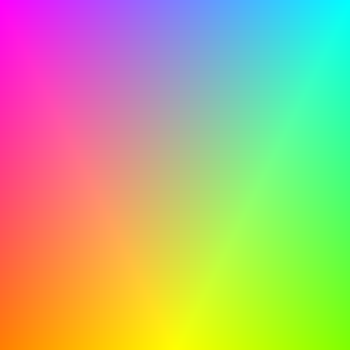
The concept of gradients isn't difficult to extend to 2D, we simply add together the result of our gradient calculations on both the X and Y positions of the pixel under consideration. Replace our original img.putdata routine with this block of code.
pixels = []
for y in range(256):
    for x in range(256):
        pixels.append(tuple(sum(
            np.array(gradient(stops, t))
            for stops, t in zip(
                [
                    [
                        (0, np.array([255,   0,   0])),
                        (1, np.array([  0, 255,   0])),
                    ], [
                        (0, np.array([  0,   0, 255])),
                        (1, np.array([128, 128,   0])),
                    ]
                ],
                (x/256, y/256)
            )
        )))
img.putdata(pixels)
Look at the absolutely beautiful rainbow gradient it produces. Look at how perfectly smooth it is! It's amazing how the image came from just a couple dozen lines of straightforward code.
Radial gradients use the distance from an origin to the X-Y position of the pixel under consideration as the timestep. At this point it's probably a good idea to replace the magic number "256" with meaningful variable names like WIDTH and HEIGHT, in case you want to change the output resolution. I define a new function hexcolor() that converts hex colors to RGB values. This makes color adjustments easier. I wrote both a version that processes strings and one that processes actual hex numbers. Use whichever one you prefer.
# def hexcolor(n):
#     return np.array([
#         (n&0xff0000) >> 16,
#         (n&0x00ff00) >>  8,
#         (n&0x0000ff) >>  0,
#     ])

def hexcolor(s):
    assert len(s) == 6
    return np.array([
        int(s[0:2], base=16),
        int(s[2:4], base=16),
        int(s[4:6], base=16),
    ])

pixels = []
for y in range(256):
    for x in range(256):
        pixels.append(tuple(sum(
            np.array(gradient(stops,
                min(1, math.sqrt(
                    (x/256 - cx)**2 +
                    (y/256 - cy)**2
                ))
            ))
            for (cx, cy), *stops in [
                [
                    (.5, .5),
                    ( 0, hexcolor('ff8c00')),
                    (.5, hexcolor('ffd700')),
                    ( 1, hexcolor('ffd700')),
                ], [
                    (.5, .5),
                    ( 0, hexcolor('ff0000')),
                    (.1, hexcolor('ff0000')),
                    (.1, hexcolor('ffffff')),
                    (.2, hexcolor('ffffff')),
                    (.2, hexcolor('ff0000')),
                    (.3, hexcolor('ff0000')),
                    (.3, hexcolor('ffffff')),
                    (.4, hexcolor('ffffff')),
                    (.4, hexcolor('ff0000')),
                    ( 1, hexcolor('ff0000')),
                ],
            ]
        )))
img.putdata(pixels)
It produces a target blended with an orange gradient. The edges are jagged, and if that's a problem for you try implementing supersampling or some other antialiasing method.

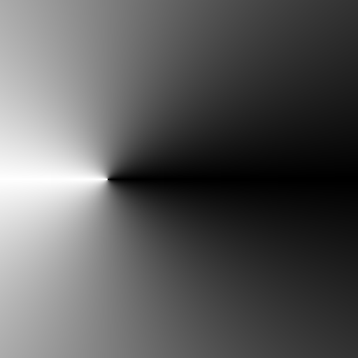
Conic gradients are the same concept but use the angle against the X-axis from a line drawn from the origin to the X-Y position of the pixel under consideration.
pixels = []
for y in range(256):
    for x in range(256):
        pixels.append(tuple(sum(
            np.array(gradient(stops,
                abs(math.atan2(y/256 - cy, x/256 - cx)) / (math.pi*2)
            ))
            for (cx, cy), *stops in [
                [
                    (.3, .5),
                    ( 0, hexcolor('000000')),
                    (.5, hexcolor('ffffff')),
                    ( 1, hexcolor('000000')),
                ],
            ]
        )))
img.putdata(pixels)
For radial and conic gradients we're essentially converting Cartesian to polar coordinates and using either the distance or the azimuth/angle as the timestep. It can also be thought of as expressing a complex number in polar form. The code for conic gradients produces a sort of 3D cone viewed from directly above with a light source to the left.
Throughout this post you might've seen bands of color or other distortions on the images. That's a result of JPEG compression artifacts and is not a fault of the code.
Exercises for the Reader
If you want something to do, you can extend the code to interpolate based off of an arbitrary Bézier curve. Maybe check out a primer, the Wikipedia article, and non-boring gradients if you want to set out on that endeavour. I didn't mention speed, but the code for calculating certain gradients run painfully slowly—try optimizing the code.